|
PythonPlaza -
Python & AI
|
Supervised Machine Learning Algorithms
Gradient Boosting
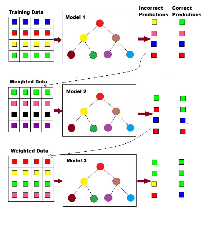
A machine learning method called Gradient Boosting creates an ensemble by combining several weak prediction models. Decision trees, which are sequentially trained to reduce errors and increase accuracy, are commonly used as these weak models. Gradient boosting can efficiently capture intricate correlations between features by combining several decision tree regressors or decision tree classifiers.
Gradient boosting's capacity to iteratively minimize the loss function is one of its main advantages. One loss function used to assess how well a machine learning model matches actual data is Mean Squared Error (MSE). MSE determines the mean of the squared discrepancies between the observed and expected values.
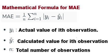
MAE (Mean Absolute Error) quantifies the average magnitude of errors for Gradient Boosting Regression.
Mean Absolute Error
It calculates the average discrepancy between a dataset's actual and forecasted values. Without taking direction into account, it displays the deviation between predicted and actual values.
1. Determined by utilizing absolute differences
2. Easy to calculate and understand
3. Handles every mistake equally
4. Not as susceptible to significant errors as MSE
5. Frequently employed to assess regression models
 USE CASE 1: Use Gradient Boosting with scikit-learn, predict the product price. The Production cost, Advertising spend, and Demand level are the independent variables.
import pandas as pd
from sklearn.model_selection import train_test_split
from sklearn.ensemble import GradientBoostingRegressor
from sklearn.metrics import mean_absolute_error, r2_score

# -----------------------------------
# 1. Load data from Excel
# -----------------------------------
data = pd.read_excel("product_data.xlsx")

print("Dataset Preview:")
print(data.head())

# -----------------------------------
# 2. Define features and target
# -----------------------------------
X = data[['Production_Cost', 'Advertising_Spend', 'Demand_Level']]
y = data['Product_Price']

# -----------------------------------
# 3. Split into training and testing
# -----------------------------------
X_train, X_test, y_train, y_test = train_test_split(
    X, y, test_size=0.25, random_state=42
)

## What is random_state?

#train_test_split randomly shuffles the dataset before splitting.
#Without random_state:
#Each run → different split
#Model performance changes slightly
#With random_state=42:
#Same rows go to train/test every time
#Results are reproducible


# -----------------------------------
# 4: Train the Gradient Boosting model
# -----------------------------------

model = GradientBoostingRegressor(
    n_estimators=200,
    learning_rate=0.05,
    max_depth=3,
    random_state=42
)

model.fit(X_train, y_train)


# -----------------------------------
# 5: Make predictions & evaluate
# -----------------------------------
y_pred = model.predict(X_test)

print("MAE:", mean_absolute_error(y_test, y_pred))
print("R² score:", r2_score(y_test, y_pred))

# -----------------------------------
# 6. Predict price for a new product
# -----------------------------------
new_product = [[65, 18, 275]]  # Production Cost, Advertising Spend, Demand Level
predicted_price = model.predict(new_product)

print("Predicted Product Price:", predicted_price[0])
USE CASE 2: Use Gradient Boosting with scikit-learn to predict the Student Grade. The 'Hours_Studied, 'Attendance_%', 'Previous_Score' are the independent variables.
import numpy as np
from sklearn.model_selection import train_test_split
from sklearn.ensemble import GradientBoostingRegressor
from sklearn.metrics import mean_absolute_error, r2_score
# -----------------------------------
# 1. Load data from Excel
# -----------------------------------
#sample data can be exported to
#excel from the URL
# https://pythonPlaza.com/linear_school_grade_data.html

data = pd.read_excel("student_data.xlsx")

print("Dataset Preview:")
print(data.head())

# -----------------------------------
# 2. Define features and target
# -----------------------------------
X = data[['Hours_Studied', 'Attendance_%', 'Previous_Score']]
y = data['Final_Grade']

# -----------------------------------
# 3. Split into training and testing
# -----------------------------------
X_train, X_test, y_train, y_test = train_test_split(
    X, y, test_size=0.25, random_state=42
)

## What is random_state?

#train_test_split randomly shuffles the dataset before splitting.
#Without random_state:
#Each run → different split
#Model performance changes slightly
#With random_state=42:
#Same rows go to train/test every time
#Results are reproducible


# -----------------------------------
# 4: Train the Gradient Boosting model
# -----------------------------------

model = GradientBoostingRegressor(
    n_estimators=200,
    learning_rate=0.05,
    max_depth=3,
    random_state=42
)

model.fit(X_train, y_train)


# -----------------------------------
# 5: Make predictions & evaluate
# -----------------------------------
y_pred = model.predict(X_test)

print("MAE:", mean_absolute_error(y_test, y_pred))
print("R² score:", r2_score(y_test, y_pred))

Example: Predict a new student’s grade
# New student: [hours_studied, attendance %, previous_score]
new_student = np.array([[6, 85, 78]])

predicted_grade = model.predict(new_student)
print("Predicted final grade:", predicted_grade[0])
USE CASE 3: Use Gradient Boosting with scikit-learn to predict the Profit Optimization. The Price (P), Advertising (A), Units Sold (Q) are the independent variables, and Profit is the dependent variable.
import numpy as np
from sklearn.model_selection import train_test_split
from sklearn.ensemble import GradientBoostingRegressor
from sklearn.metrics import mean_absolute_error, r2_score

# -----------------------------------
# 1. Load data from Excel
# -----------------------------------
#sample data can be exported to
#excel from the URL


  Get the Profit Optimization data in Excel


data = pd.read_excel("profit_optimization.xlsx")

print("Dataset Preview:")
print(data.head())

# -----------------------------------
# 2. Define features and target  Price (P)
# -----------------------------------
X = data[['Price', 'Advertising', 'Units_Sold']]
y = data['Profit']

# -----------------------------------
# 3. Split into training and testing
# -----------------------------------
X_train, X_test, y_train, y_test = train_test_split(
    X, y, test_size=0.25, random_state=42
)

## What is random_state?

#train_test_split randomly shuffles the dataset before splitting.
#Without random_state:
#Each run → different split
#Model performance changes slightly
#With random_state=42:
#Same rows go to train/test every time
#Results are reproducible


# -----------------------------------
# 4: Train the Gradient Boosting model
# -----------------------------------

model = GradientBoostingRegressor(
    n_estimators=200,
    learning_rate=0.05,
    max_depth=3,
    random_state=42
)

model.fit(X_train, y_train)


# -----------------------------------
# 5: Make predictions & evaluate
# -----------------------------------
y_pred = model.predict(X_test)

print("MAE:", mean_absolute_error(y_test, y_pred))
print("R² score:", r2_score(y_test, y_pred))


#Predict profit for a new business strategy
# Example: Price = 15, Advertising = 165, Units Sold = 460
new_strategy = np.array([[15, 165, 460]])

predicted_profit = model.predict(new_strategy)
print("Predicted profit:", predicted_profit[0])
USE CASE 4: Use Gradient Boosting with scikit-learn to predict the Patient Response. The Dosage (mg), Age (yrs), Weight (lbs) are the independent variables, and Patient Response is the dependent variable.
import numpy as np
from sklearn.model_selection import train_test_split
from sklearn.ensemble import GradientBoostingRegressor
from sklearn.metrics import mean_absolute_error, r2_score

# -----------------------------------
# 1. Load data from Excel
# -----------------------------------
#sample data can be exported to
#excel from the URL


  Get the Patient Response Data in Excel


data = pd.read_excel("patient_dosage_response.xlsx")

print("Dataset Preview:")
print(data.head())

# -----------------------------------
# 2. Define features and target  Price (P)
# -----------------------------------
X = data[['Dosage', 'Age', 'Weight']]
y = data['Patient_Response']

# -----------------------------------
# 3. Split into training and testing
# -----------------------------------
X_train, X_test, y_train, y_test = train_test_split(
    X, y, test_size=0.25, random_state=42
)

## What is random_state?

#train_test_split randomly shuffles the dataset before splitting.
#Without random_state:
#Each run → different split
#Model performance changes slightly
#With random_state=42:
#Same rows go to train/test every time
#Results are reproducible

# -----------------------------------
# 4: Train the Gradient Boosting model
# -----------------------------------

model = GradientBoostingRegressor(
    n_estimators=200,
    learning_rate=0.05,
    max_depth=3,
    random_state=42
)


model.fit(X_train, y_train)


# -----------------------------------
# 5: Make predictions & evaluate
# -----------------------------------
y_pred = model.predict(X_test)

print("MAE:", mean_absolute_error(y_test, y_pred))
print("R² score:", r2_score(y_test, y_pred))

#Predict response for a new patient
# New patient: Dosage=72mg, Age=36yrs, Weight=172lbs
new_patient = np.array([[72, 36, 172]])

#predicted_response = model.predict(new_patient)
print("Predicted patient response:", predicted_response[0])
About Us | Contact Us | Sitemap | Privacy Policy