Decision Trees (Classification Algorithm)

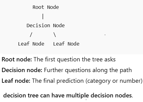
The decision tree is called that because it creates models for classification or prediction in the shape of a tree. It splits the data into smaller parts and connects each part with a decision. This makes a tree with decision points and final answers. A decision point can have two or more paths and leads to the final answers. A final answer shows the result of the classification or decision. It uses the if-then-else rule to make predictions. As you go deeper into the tree, the rules get more complicated, which makes the model more accurate. A decision tree has:

Root Node: The process starts at the top of the tree with the entire dataset.
Internal Nodes (Decision Nodes): At each internal node, the algorithm tests a specific attribute or feature to split the data into smaller, more homogeneous subsets.
Leaf Nodes (Terminal Nodes): The process ends at the leaf nodes, which represent the final decision, class label, or predicted continuous value.

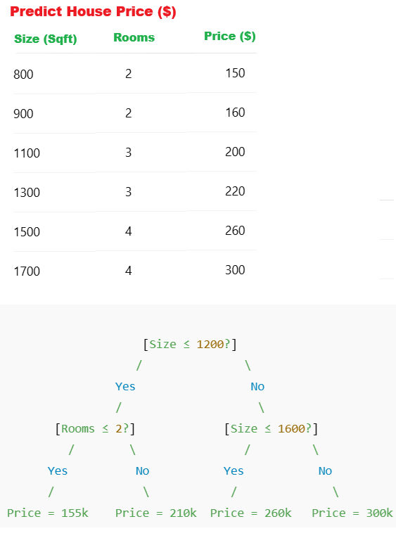
Let's see an example

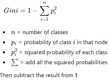
Gini Impurity

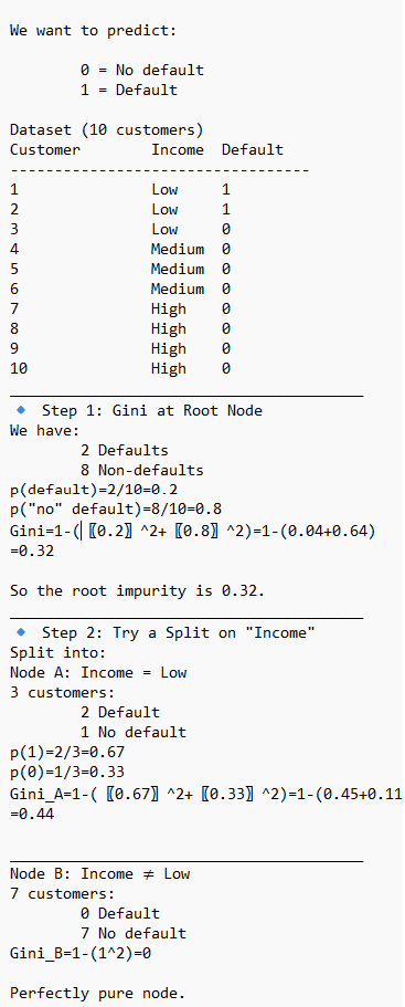
Gini Impurity is commonly used in Decision trees, Random Forest, primarily as the default criterion to measure the quality of splits in the individual classification trees. It calculates how frequently a randomly chosen element would be incorrectly labeled, guiding the algorithm to create pure, homogeneous nodes.
Node Splitting: During tree construction, the algorithm calculates the Gini Impurity for possible splits, choosing the one that minimizes impurity.

USE CASE 1: Using Decision Tree with scikit-learn, predict the product price. The Production cost, Advertising spend, and Demand level are the independent variables.

import pandas as pd
from sklearn.tree import DecisionTreeRegressor
from sklearn.model_selection import train_test_split
from sklearn.metrics import mean_absolute_error, r2_score

# -----------------------------------
# 1. Load data from Excel
# -----------------------------------
data = pd.read_excel("product_data.xlsx")

print("Dataset Preview:")
print(data.head())

# -----------------------------------
# 2. Define features and target
# -----------------------------------
X = data[['Production_Cost', 'Advertising_Spend', 'Demand_Level']]
y = data['Product_Price']

# -----------------------------------
# 3. Split into training and testing
# -----------------------------------
X_train, X_test, y_train, y_test = train_test_split(
    X, y, test_size=0.25, random_state=42
)

# -----------------------------------
# 4. Train the Decision Tree model
# -----------------------------------
model = DecisionTreeRegressor(
    max_depth=4,
    random_state=42
)


## What is random_state?

#train_test_split randomly shuffles the dataset before splitting.
#Without random_state:
#Each run → different split
#Model performance changes slightly
#With random_state=42:
#Same rows go to train/test every time
#Results are reproducible


model.fit(X_train, y_train)



# -----------------------------------
# 6. Evaluate the model
# -----------------------------------
y_pred = model.predict(X_test)

print("MAE:", mean_absolute_error(y_test, y_pred))
print("R² score:", r2_score(y_test, y_pred))


# -----------------------------------
# 7. Predict price for a new product
# -----------------------------------
new_product = pd.DataFrame({
    'Production_Cost': [68],
    'Advertising_Spend': [13],
    'Demand_Level': [37]
})

predicted_price = model.predict(new_product)

print("\nPredicted Product Price:", predicted_price[0])

import numpy as np
from sklearn.model_selection import train_test_split
from sklearn.tree import DecisionTreeRegressor
from sklearn.metrics import mean_absolute_error, r2_score

# -----------------------------------
# 1. Load data from Excel
# -----------------------------------
#sample data can be exported to 
#excel from the URL
# https://pythonPlaza.com/linear_school_grade_data.html

data = pd.read_excel("student_data.xlsx")

print("Dataset Preview:")
print(data.head())

# -----------------------------------
# 2. Define features and target
# -----------------------------------
X = data[['Hours_Studied', 'Attendance_%', 'Previous_Score']]
y = data['Final_Grade']

# -----------------------------------
# 3. Split into training and testing
# -----------------------------------
X_train, X_test, y_train, y_test = train_test_split(
    X, y, test_size=0.25, random_state=42
)


# -----------------------------------
# 4. Train the Decision Tree model
# -----------------------------------
model = DecisionTreeRegressor(
    max_depth=4,
    random_state=42
)


## What is random_state?

#train_test_split randomly shuffles the dataset before splitting.
#Without random_state:
#Each run → different split
#Model performance changes slightly
#With random_state=42:
#Same rows go to train/test every time
#Results are reproducible


model.fit(X_train, y_train)

# -----------------------------------
# 6. Evaluate the model
# -----------------------------------
y_pred = model.predict(X_test)

print("MAE:", mean_absolute_error(y_test, y_pred))
print("R² score:", r2_score(y_test, y_pred))


Example: Predict a new student’s grade
# New student: [hours_studied, attendance %, previous_score]
new_student = np.array([[6, 85, 78]])

predicted_grade = model.predict(new_student)
print("Predicted final grade:", predicted_grade[0])

import numpy as np
from sklearn.model_selection import train_test_split
from sklearn.tree import DecisionTreeRegressor
from sklearn.metrics import mean_absolute_error, r2_score

# -----------------------------------
# 1. Load data from Excel
# -----------------------------------
#sample data can be exported to 
#excel from the URL

  
  Get the Profit Optimization data in Excel
  

data = pd.read_excel("profit_optimization.xlsx")

print("Dataset Preview:")
print(data.head())

# -----------------------------------
# 2. Define features and target  Price (P)	
# -----------------------------------
X = data[['Price', 'Advertising', 'Units_Sold']]
y = data['Profit']

# -----------------------------------
# 3. Split into training and testing
# -----------------------------------
X_train, X_test, y_train, y_test = train_test_split(
    X, y, test_size=0.25, random_state=42
)


# -----------------------------------
# 4. Train the Decision Tree model
# -----------------------------------
model = DecisionTreeRegressor(
    max_depth=4,
    random_state=42
)


## What is random_state?

#train_test_split randomly shuffles the dataset before splitting.
#Without random_state:
#Each run → different split
#Model performance changes slightly
#With random_state=42:
#Same rows go to train/test every time
#Results are reproducible


model.fit(X_train, y_train)

# -----------------------------------
# 6. Evaluate the model
# -----------------------------------
y_pred = model.predict(X_test)

print("MAE:", mean_absolute_error(y_test, y_pred))
print("R² score:", r2_score(y_test, y_pred))


#Predict profit for a new business strategy
# Example: Price = 15, Advertising = 165, Units Sold = 460
new_strategy = np.array([[15, 165, 460]])

predicted_profit = model.predict(new_strategy)
print("Predicted profit:", predicted_profit[0])

import numpy as np
from sklearn.model_selection import train_test_split
from sklearn.tree import DecisionTreeRegressor
from sklearn.metrics import mean_absolute_error, r2_score

# -----------------------------------
# 1. Load data from Excel
# -----------------------------------
#sample data can be exported to 
#excel from the URL

  
  Get the Patient Response Data in Excel
  

data = pd.read_excel("patient_dosage_response.xlsx")

print("Dataset Preview:")
print(data.head())

# -----------------------------------
# 2. Define features and target  Price (P)	
# -----------------------------------
X = data[['Dosage', 'Age', 'Weight']]
y = data['Patient_Response']

# -----------------------------------
# 3. Split into training and testing
# -----------------------------------
X_train, X_test, y_train, y_test = train_test_split(
    X, y, test_size=0.25, random_state=42
)


# -----------------------------------
# 4. Train the Decision Tree model
# -----------------------------------
model = DecisionTreeRegressor(
    max_depth=4,
    random_state=42
)


## What is random_state?

#train_test_split randomly shuffles the dataset before splitting.
#Without random_state:
#Each run → different split
#Model performance changes slightly
#With random_state=42:
#Same rows go to train/test every time
#Results are reproducible


model.fit(X_train, y_train)



# -----------------------------------
# 6. Evaluate the model
# -----------------------------------
y_pred = model.predict(X_test)

print("MAE:", mean_absolute_error(y_test, y_pred))
print("R² score:", r2_score(y_test, y_pred))

Predict response for a new patient
# New patient: Dosage=72mg, Age=36yrs, Weight=172lbs
new_patient = np.array([[72, 36, 172]])

predicted_response = model.predict(new_patient)
print("Predicted patient response:", predicted_response[0])