|
PythonPlaza -
Python & AI
|
Supervised Machine Learning Algorithms
Random Forest (Regression Algorithm)
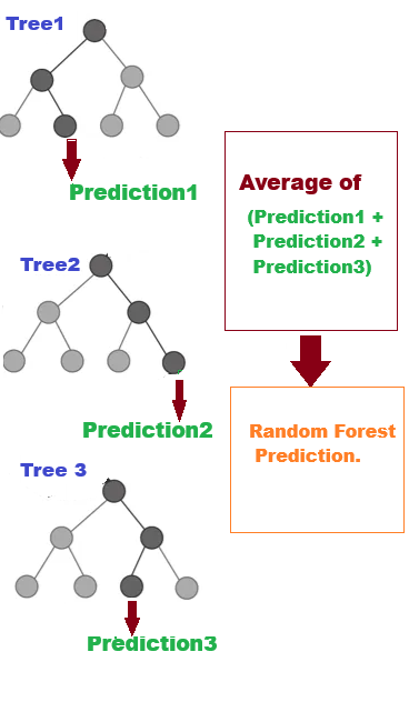
Random Forest is a machine learning algorithm that creates many decision trees with various subsets data. Each tree can have a different root node. The method uses these trees to make predictions by randomly looking at different parts of the data. For classification tasks, the final answer is chosen based on what most trees agree on. For regression tasks, the result is the average of all the trees' predictions. This method is called ensemble learning, which helps make predictions more accurate and reduces mistakes. The way the trees are built, including their root and decision points, makes Random Forest powerful and less likely to learn from the training data too closely.
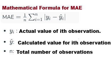
Minimizing the Error: Mean Absolute Error
The mean absolute error calculates the average discrepancy between a dataset's actual and projected values. Without taking direction into account, it displays the deviation between predicted and actual values.
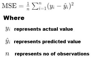
Minimizing the Error: Mean Squared Error (MSE)
A key idea in statistics and machine learning, mean squared error (MSE) is essential for evaluating the precision of predictive models.
The model's accuracy can be examined using the MSE value.It calculates the average squared difference between the dataset's actual and projected values.
It is computed by averaging the squared residuals, where the residual is the difference between each data point's actual value and its anticipated value.
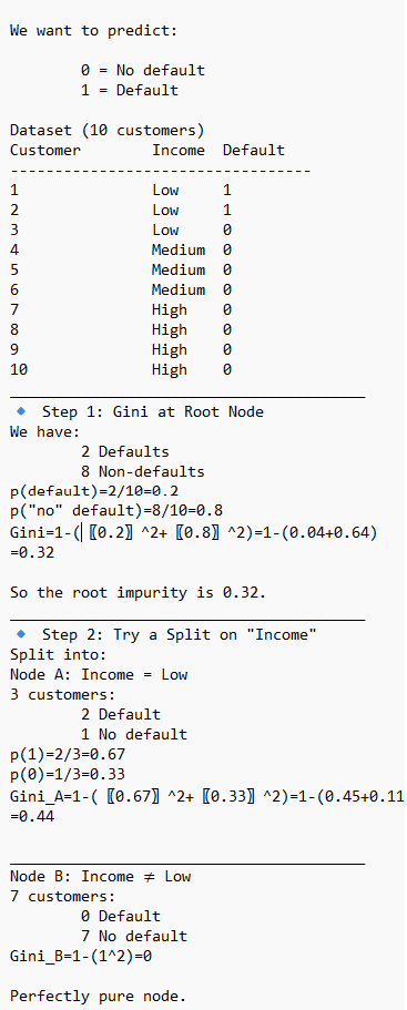
 Gini Impurity
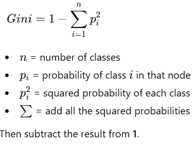
Gini Impurity is commonly used in Decision trees, Random Forest, primarily as the default criterion to measure the quality of splits in the individual classification trees. It calculates how frequently a randomly chosen element would be incorrectly labeled, guiding the algorithm to create pure, homogeneous nodes.
Node Splitting: During tree construction, the algorithm calculates the Gini Impurity for possible splits, choosing the one that minimizes impurity.
 USE CASE 1: Use Random Forest with scikit-learn, predict the product price. The Production cost, Advertising spend, and Demand level are the independent variables.
import pandas as pd
import numpy as np
from sklearn.model_selection import train_test_split
from sklearn.ensemble import RandomForestRegressor
from sklearn.metrics import mean_absolute_error, r2_score
# -----------------------------------
# 1. Load data from Excel
# -----------------------------------
data = pd.read_excel("product_data.xlsx")

print("Dataset Preview:")
print(data.head())

# -----------------------------------
# 2. Define features and target
# -----------------------------------
X = data[['Production_Cost', 'Advertising_Spend', 'Demand_Level']]
y = data['Product_Price']

# -----------------------------------
# 3. Split into training and testing
# -----------------------------------
X_train, X_test, y_train, y_test = train_test_split(
    X, y, test_size=0.25, random_state=42
)

## What is random_state?

#train_test_split randomly shuffles the dataset before splitting.
#Without random_state:
#Each run → different split
#Model performance changes slightly
#With random_state=42:
#Same rows go to train/test every time
#Results are reproducible

# -----------------------------------
# 4. Train the Random Forest model
# -----------------------------------
model = RandomForestRegressor(
    n_estimators=200,
    max_depth=6,
    random_state=42
)

model.fit(X_train, y_train)

# -----------------------------------
# 5. Make predictions & evaluate
# -----------------------------------
y_pred = model.predict(X_test)

print("MAE:", mean_absolute_error(y_test, y_pred))
print("R² score:", r2_score(y_test, y_pred))


# -----------------------------------
# 6. Predict price for a new product
# -----------------------------------
# New product: Cost=32, Advertising=160, Demand=62
new_product = np.array([[32, 160, 62]])

predicted_price = model.predict(new_product)
print("Predicted product price:", predicted_price[0])

Why Random Forest works well here

1. It captures non-linear relationships very well.
2. It handles feature interactions automatically.
3. It is more robust than a single decision tree.
4. It reduces overfitting by averaging.
USE CASE 2: Use Random Forest with scikit-learn to predict the Student Grade. The 'Hours_Studied, 'Attendance_%', 'Previous_Score' are the independent variables.
import numpy as np
from sklearn.model_selection import train_test_split
from sklearn.ensemble import RandomForestRegressor
from sklearn.metrics import mean_absolute_error, r2_score

# -----------------------------------
# 1. Load data from Excel
# -----------------------------------
#sample data can be exported to
#excel from the URL
# https://pythonPlaza.com/linear_school_grade_data.html

data = pd.read_excel("student_data.xlsx")

print("Dataset Preview:")
print(data.head())

# -----------------------------------
# 2. Define features and target
# -----------------------------------
X = data[['Hours_Studied', 'Attendance_%', 'Previous_Score']]
y = data['Final_Grade']

# -----------------------------------
# 3. Split into training and testing
# -----------------------------------
X_train, X_test, y_train, y_test = train_test_split(
    X, y, test_size=0.25, random_state=42
)

# -----------------------------------
# 4. Train the Random Forest model
# -----------------------------------
model = RandomForestRegressor(
    n_estimators=200,
    max_depth=6,
    random_state=42
)


## What is random_state?

#train_test_split randomly shuffles the dataset before splitting.
#Without random_state:
#Each run → different split
#Model performance changes slightly
#With random_state=42:
#Same rows go to train/test every time
#Results are reproducible

model.fit(X_train, y_train)

# -----------------------------------
# 5. Make predictions & evaluate
# -----------------------------------
y_pred = model.predict(X_test)

print("MAE:", mean_absolute_error(y_test, y_pred))
print("R² score:", r2_score(y_test, y_pred))

Example: Predict a new student’s grade
# New student: [hours_studied, attendance %, previous_score]
new_student = np.array([[6, 85, 78]])

predicted_grade = model.predict(new_student)
print("Predicted final grade:", predicted_grade[0])
USE CASE 3: Use Random Forest with scikit-learn to predict the Profit Optimization. The Price (P), Advertising (A), Units Sold (Q) are the independent variables, and Profit is the dependent variable.
import numpy as np
from sklearn.model_selection import train_test_split
from sklearn.ensemble import RandomForestRegressor
from sklearn.metrics import mean_absolute_error, r2_score

# -----------------------------------
# 1. Load data from Excel
# -----------------------------------
#sample data can be exported to
#excel from the URL


  Get the Profit Optimization data in Excel


data = pd.read_excel("profit_optimization.xlsx")

print("Dataset Preview:")
print(data.head())

# -----------------------------------
# 2. Define features and target  Price (P)
# -----------------------------------
X = data[['Price', 'Advertising', 'Units_Sold']]
y = data['Profit']

# -----------------------------------
# 3. Split into training and testing
# -----------------------------------
X_train, X_test, y_train, y_test = train_test_split(
    X, y, test_size=0.25, random_state=42
)

# -----------------------------------
# 4. Train the Random Forest model
# -----------------------------------
model = RandomForestRegressor(
    n_estimators=200,
    max_depth=6,
    random_state=42
)


## What is random_state?

#train_test_split randomly shuffles the dataset before splitting.
#Without random_state:
#Each run → different split
#Model performance changes slightly
#With random_state=42:
#Same rows go to train/test every time
#Results are reproducible

model.fit(X_train, y_train)

# -----------------------------------
# 5. Make predictions & evaluate
# -----------------------------------
y_pred = model.predict(X_test)

print("MAE:", mean_absolute_error(y_test, y_pred))
print("R² score:", r2_score(y_test, y_pred))

#Predict profit for a new business strategy
# Example: Price = 15, Advertising = 165, Units Sold = 460
new_strategy = np.array([[15, 165, 460]])

predicted_profit = model.predict(new_strategy)
print("Predicted profit:", predicted_profit[0])
USE CASE 4: Use Random Forest with scikit-learn to predict the Patient Response. The Dosage (mg), Age (yrs), Weight (lbs) are the independent variables, and Patient Response is the dependent variable.
import numpy as np
from sklearn.model_selection import train_test_split
from sklearn.ensemble import RandomForestRegressor
from sklearn.metrics import mean_absolute_error, r2_score

# -----------------------------------
# 1. Load data from Excel
# -----------------------------------
#sample data can be exported to
#excel from the URL


  Get the Patient Response Data in Excel


data = pd.read_excel("patient_dosage_response.xlsx")

print("Dataset Preview:")
print(data.head())

# -----------------------------------
# 2. Define features and target  Price (P)
# -----------------------------------
X = data[['Dosage', 'Age', 'Weight']]
y = data['Patient_Response']

# -----------------------------------
# 3. Split into training and testing
# -----------------------------------
X_train, X_test, y_train, y_test = train_test_split(
    X, y, test_size=0.25, random_state=42
)

# -----------------------------------
# 4. Train the Random Forest model
# -----------------------------------
model = RandomForestRegressor(
    n_estimators=200,
    max_depth=6,
    random_state=42
)


## What is random_state?

#train_test_split randomly shuffles the dataset before splitting.
#Without random_state:
#Each run → different split
#Model performance changes slightly
#With random_state=42:
#Same rows go to train/test every time
#Results are reproducible

model.fit(X_train, y_train)

# -----------------------------------
# 5. Make predictions & evaluate
# -----------------------------------
y_pred = model.predict(X_test)

print("MAE:", mean_absolute_error(y_test, y_pred))
print("R² score:", r2_score(y_test, y_pred))


Predict response for a new patient
# New patient: Dosage=72mg, Age=36yrs, Weight=172lbs
new_patient = np.array([[72, 36, 172]])

predicted_response = model.predict(new_patient)
print("Predicted patient response:", predicted_response[0])
About Us | Contact Us | Sitemap | Privacy Policy