PythonPlaza.com

Support Vector Machine(SVM)

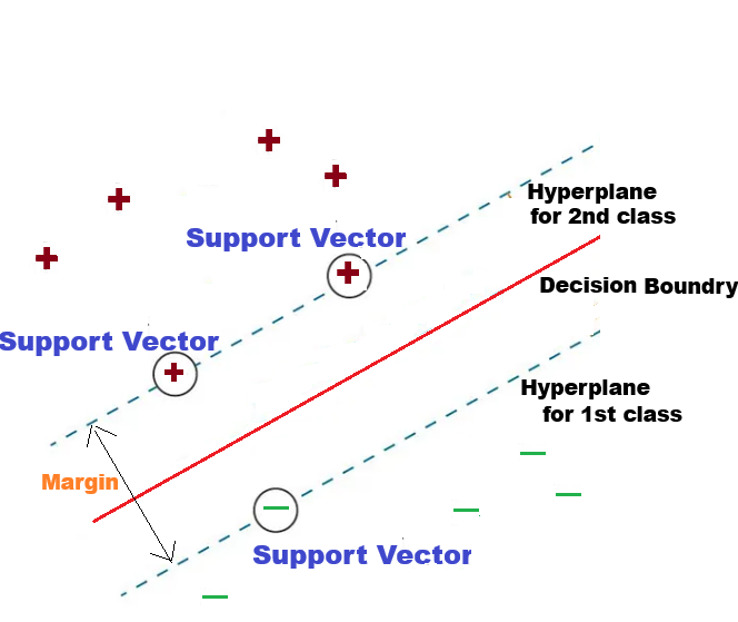
Support Vector Machine, or SVM, is a type of machine learning that is used for both classification and regression. It works by finding the best line, called a Decision Boundary that separates different groups in the data. SVM is helpful when you need to sort things into two groups, like identifying if an email is spam or not, or if an image is of a cat or a dog.

Support vectors are the key points in the data that are closest to the line that separates the groups. The margin is the space between this line and the nearest points from each group.

The support vectors do not just help generate the decision boundary—they completely dictate it. Every other data point in your dataset can be modified, moved around, or deleted entirely, and the decision boundary will remain exactly the same, as long as the support vectors do not change.

The Decision Boundary is the strict dividing line between the two categories. Everything on one side of the decision boundary belongs to Category 1, and everything on the other side belongs to Category 2

The objective of a Support Vector Machine (SVM) is to maximize the distance between the nearest data points and the decision border. We refer to this distance as the margin.

How SVM Operates

The median line or plane that divides the data into classes is known as the decision boundary. Each class's closest points are traversed by the hyperplanes, also known as support vectors.
The model is safer and less prone to errors on fresh data when the margin is higher. The Significance of Maximum Margin. It makes the difference between classes obvious.
It prevents the model from fitting the training set too closely. It improves the model's performance on test data.

Support Vector Regression (SVR)

A step-by-step housing price example using 15 observations

Please note: For determining the weights → points inside the tube don't directly contribute

1. Why Support Vector Regression?

A standard Support Vector Machine (SVM) is commonly introduced as a classification algorithm. For example, classification predicts whether an observation belongs to one of two classes:

\[ y \in \{-1,+1\} \]

However, house price is a continuous variable. Therefore, instead of ordinary SVM classification, we use Support Vector Regression (SVR).

Key idea: SVR tries to find a regression function that predicts house prices while allowing small errors inside an $ \epsilon $-tube.

2. Housing Dataset

We will use three predictors:

$x_1$ = house size in 1000 square feet
$x_2$ = number of bedrooms
$x_3$ = house age in years
$y$ = house price in units of $100,000

House	Size $x_1$	Bedrooms $x_2$	Age $x_3$	Price $y$
1	1.0	2	30	2.20
2	1.2	2	25	2.50
3	1.4	3	20	3.00
4	1.5	3	15	3.30
5	1.7	3	12	3.60
6	1.8	4	10	4.00
7	2.0	4	8	4.40
8	2.1	4	5	4.70
9	2.3	4	7	5.00
10	2.5	5	5	5.50
11	2.7	5	4	5.90
12	2.8	5	3	6.20
13	3.0	5	2	6.60
14	3.2	6	2	7.00
15	3.5	6	1	7.50

The goal is to estimate a house's price from its size, number of bedrooms, and age.

3. The SVR Regression Function

The simplest linear SVR model is:

\[ \boxed{ f(x)=w_1x_1+w_2x_2+w_3x_3+b } \]

where:

$w_1,w_2,w_3$ are the weights
$b$ is the intercept
$x_1,x_2,x_3$ are the house characteristics

Example weights

Suppose, for illustration, that:

\[ w_1=1.5,\qquad w_2=0.3,\qquad w_3=-0.02,\qquad b=0.5 \]

Then our prediction equation becomes:

\[ \boxed{ f(x)=1.5x_1+0.3x_2-0.02x_3+0.5 } \]

4. The $ \epsilon $-Tube

SVR does not try to make every prediction exactly equal to the actual house price.

Instead, it creates a tube around the regression function:

\[ f(x)+\epsilon \]

and

\[ f(x)-\epsilon \]

Suppose:

\[ \boxed{\epsilon=0.20} \]

A prediction is considered acceptable when:

\[ \boxed{ |y-f(x)|\leq0.20 } \]

Interpretation: An error of up to 0.20 (i.e. $20,000 because our price is measured in units of $100,000) is considered acceptable and receives no SVR penalty.

5. Example: A House Inside the Tube

Suppose the actual price is:

\[ y=4.40 \]

and our model predicts:

\[ f(x)=4.30 \]

The prediction error is:

\[ |4.40-4.30|=0.10 \]

Since:

\[ 0.10<0.20 \]

Result: The observation is inside the $ \epsilon $-tube, so there is no SVR penalty.

6. Example: A House Outside the Tube

Now suppose the actual price is:

\[ y=5.00 \]

and the model predicts:

\[ f(x)=4.60 \]

The prediction error is:

\[ |5.00-4.60|=0.40 \]

Since the allowed error is $0.20$, the amount outside the tube is:

\[ 0.40-0.20=0.20 \]

Therefore, this observation produces an SVR loss of:

\[ \boxed{ L_{\epsilon} = \max(0,|y-f(x)|-\epsilon) } \]

For this house:

\[ L_{\epsilon} = \max(0,0.40-0.20) = \boxed{0.20} \]

Interpretation: The house is 0.20 units of price outside the acceptable $ \epsilon $-tube and therefore receives a penalty.

7. Slack Variables

The slack variable measures how far an observation goes beyond the $ \epsilon $-boundary.

\[ \boxed{ \xi_i=\max(0,y_i-f(x_i)-\epsilon) } \]

for an observation above the upper boundary, and:

\[ \boxed{ \xi_i^* = \max(0,f(x_i)-y_i-\epsilon) } \]

for an observation below the lower boundary.

Simple interpretation: If a point is inside the tube, its slack is zero. If it is outside the tube, the slack tells us how far outside the tube it is.

8. SVR Optimization Problem

The full mathematical form can look complicated because it uses slack variables:

\[ \min_{w,b,\xi,\xi^*} \frac12(w_1^2+w_2^2+w_3^2) + C\sum_{i=1}^{15}(\xi_i+\xi_i^*) \]

For understanding the housing example, we can write the same idea in a much simpler form:

\[ \boxed{ \min\quad \frac12(w_1^2+w_2^2+w_3^2) + C(\text{total error outside the tube}) } \]

What does this mean?

Keep the weights small

\[ \frac12(w_1^2+w_2^2+w_3^2) \]

Penalize observations outside the tube

\[ C(\text{total error outside the tube}) \]

Find the best balance

The algorithm searches for the weights and intercept that minimize the total objective.

9. Support Vectors

Not all 15 houses necessarily determine the final SVR model.

Position of observation	SVR role
Strictly inside the $ \epsilon $-tube	Usually not a support vector
On the $ \epsilon $-boundary	Can be a support vector
Outside the $ \epsilon $-tube	Support vector

Key idea: The support vectors are the observations that are important in determining the final regression function.

In the linear SVR dual formulation, the weights can be expressed as:

\[ \boxed{ w= \sum_{i=1}^{15} (\alpha_i-\alpha_i^*)x_i } \]

Therefore, an observation strictly inside the tube has:

\[ \alpha_i=\alpha_i^*=0 \]

and therefore contributes nothing directly to the calculation of $w$.

10. The Main Idea

For our 15-house housing dataset, SVR tries to find a regression function:

\[ \boxed{ f(x)=w_1x_1+w_2x_2+w_3x_3+b } \]

while minimizing:

\[ \boxed{ \frac12(w_1^2+w_2^2+w_3^2) + C\sum_{i=1}^{15} \max(0,|y_i-\hat y_i|-\epsilon) } \]

In simple words:

\[ \boxed{ \text{Minimize} = \text{small weights} + \text{penalty for errors outside the tube} } \]

Points comfortably inside the tube have zero penalty. Points on or outside the tube are the observations that can determine the regression model and become support vectors.

USE CASE 1: Using Support Vector Machine with scikit-learn, predict the product price. The Production cost, Advertising spend, and Demand level are the independent variables.

import pandas as pd from sklearn.model_selection import train_test_split from sklearn.preprocessing import StandardScaler from sklearn.svm import SVR from sklearn.metrics import mean_squared_error, r2_score # ----------------------------------- # 1. Load data from Excel # ----------------------------------- data = pd.read_excel("product_data.xlsx") print("Dataset Preview:") print(data.head()) # ----------------------------------- # Define features and target # ----------------------------------- X = data[['Production_Cost', 'Advertising_Spend', 'Demand_Level']] y = data['Product_Price'] # ----------------------------------- # Split into training and testing # ----------------------------------- X_train, X_test, y_train, y_test = train_test_split( X, y, test_size=0.25, random_state=42 ) ## What is random_state? #train_test_split randomly shuffles the dataset before splitting. #Without random_state: #Each run → different split #Model performance changes slightly #With random_state=42: #Same rows go to train/test every time #Results are reproducible #SVM is sensitive to feature magnitude, so we must standardize the data. # Scale the Features scaler = StandardScaler() X_train_scaled = scaler.fit_transform(X_train) X_test_scaled = scaler.transform(X_test) #Train the SVR Model #We’ll use an RBF kernel (most common for non-linear problems): model = SVR(kernel='rbf') model.fit(X_train_scaled, y_train) #Make Predictions y_pred = model.predict(X_test_scaled) #Evaluate the Model mse = mean_squared_error(y_test, y_pred) r2 = r2_score(y_test, y_pred) print("Mean Squared Error:", mse) print("R2 Score:", r2) # ----------------------------------- # 7. Predict price for a new product # ----------------------------------- new_product = pd.DataFrame({ 'Production_Cost': [68], 'Advertising_Spend': [13], 'Demand_Level': [37] }) predicted_price = model.predict(new_product) print("\nPredicted Product Price:", predicted_price[0])

import pandas as pd from sklearn.model_selection import train_test_split from sklearn.preprocessing import StandardScaler from sklearn.svm import SVR from sklearn.metrics import mean_squared_error, r2_score # ----------------------------------- # 1. Load data from Excel # ----------------------------------- #sample data can be exported to #excel from the URL # https://pythonPlaza.com/linear_school_grade_data.html data = pd.read_excel("student_data.xlsx") print("Dataset Preview:") print(data.head()) # ----------------------------------- # Define features and target # ----------------------------------- X = data[['Hours_Studied', 'Attendance_%', 'Previous_Score']] y = data['Final_Grade'] # ----------------------------------- # Split into training and testing # ----------------------------------- X_train, X_test, y_train, y_test = train_test_split( X, y, test_size=0.25, random_state=42 ) ## What is random_state? #train_test_split randomly shuffles the dataset before splitting. #Without random_state: #Each run → different split #Model performance changes slightly #With random_state=42: #Same rows go to train/test every time #Results are reproducible #SVM is sensitive to feature magnitude, so we must standardize the data. # Scale the Features scaler = StandardScaler() X_train_scaled = scaler.fit_transform(X_train) X_test_scaled = scaler.transform(X_test) #Train the SVR Model #We’ll use an RBF kernel (most common for non-linear problems): model = SVR(kernel='rbf') model.fit(X_train_scaled, y_train) #Make Predictions y_pred = model.predict(X_test_scaled) #Evaluate the Model mse = mean_squared_error(y_test, y_pred) r2 = r2_score(y_test, y_pred) print("Mean Squared Error:", mse) print("R2 Score:", r2) Example: Predict a new student’s grade # New student: [hours_studied, attendance %, previous_score] new_student = np.array([[6, 85, 78]]) predicted_grade = model.predict(new_student) print("Predicted final grade:", predicted_grade[0])

import pandas as pd from sklearn.model_selection import train_test_split from sklearn.preprocessing import StandardScaler from sklearn.svm import SVR from sklearn.metrics import mean_squared_error, r2_score # ----------------------------------- # 1. Load data from Excel # ----------------------------------- #sample data can be exported to #excel from the URL Get the Profit Optimization data in Excel data = pd.read_excel("profit_optimization.xlsx") print("Dataset Preview:") print(data.head()) # ----------------------------------- # Define features and target Price (P) # ----------------------------------- X = data[['Price', 'Advertising', 'Units_Sold']] y = data['Profit'] # ----------------------------------- # Split into training and testing # ----------------------------------- X_train, X_test, y_train, y_test = train_test_split( X, y, test_size=0.25, random_state=42 ) ## What is random_state? #train_test_split randomly shuffles the dataset before splitting. #Without random_state: #Each run → different split #Model performance changes slightly #With random_state=42: #Same rows go to train/test every time #Results are reproducible #SVM is sensitive to feature magnitude, so we must standardize the data. # Scale the Features scaler = StandardScaler() X_train_scaled = scaler.fit_transform(X_train) X_test_scaled = scaler.transform(X_test) #Train the SVR Model #We’ll use an RBF kernel (most common for non-linear problems): model = SVR(kernel='rbf') model.fit(X_train_scaled, y_train) #Make Predictions y_pred = model.predict(X_test_scaled) #Evaluate the Model mse = mean_squared_error(y_test, y_pred) r2 = r2_score(y_test, y_pred) print("Mean Squared Error:", mse) print("R2 Score:", r2) #Predict profit for a new business strategy # Example: Price = 15, Advertising = 165, Units Sold = 460 new_strategy = np.array([[15, 165, 460]]) predicted_profit = model.predict(new_strategy) print("Predicted profit:", predicted_profit[0])

import pandas as pd from sklearn.model_selection import train_test_split from sklearn.preprocessing import StandardScaler from sklearn.svm import SVR from sklearn.metrics import mean_squared_error, r2_score # ----------------------------------- # 1. Load data from Excel # ----------------------------------- #sample data can be exported to #excel from the URL Get the Patient Response Data in Excel data = pd.read_excel("patient_dosage_response.xlsx") print("Dataset Preview:") print(data.head()) # ----------------------------------- # Define features and target Price (P) # ----------------------------------- X = data[['Dosage', 'Age', 'Weight']] y = data['Patient_Response'] # ----------------------------------- # Split into training and testing # ----------------------------------- X_train, X_test, y_train, y_test = train_test_split( X, y, test_size=0.25, random_state=42 ) ## What is random_state? #train_test_split randomly shuffles the dataset before splitting. #Without random_state: #Each run → different split #Model performance changes slightly #With random_state=42: #Same rows go to train/test every time #Results are reproducible #SVM is sensitive to feature magnitude, so we must standardize the data. # Scale the Features scaler = StandardScaler() X_train_scaled = scaler.fit_transform(X_train) X_test_scaled = scaler.transform(X_test) #Train the SVR Model #We’ll use an RBF kernel (most common for non-linear problems): model = SVR(kernel='rbf') model.fit(X_train_scaled, y_train) #Make Predictions y_pred = model.predict(X_test_scaled) #Evaluate the Model mse = mean_squared_error(y_test, y_pred) r2 = r2_score(y_test, y_pred) print("Mean Squared Error:", mse) print("R2 Score:", r2) Predict response for a new patient # New patient: Dosage=72mg, Age=36yrs, Weight=172lbs new_patient = np.array([[72, 36, 172]]) predicted_response = model.predict(new_patient) print("Predicted patient response:", predicted_response[0])

Supervised Machine Learning Algorithms